NeRF
Network structure
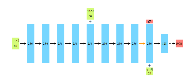
- Input vectors are shown in green(there is an embedding operation)
- intermediate hidden layers are shown in blue
- output vectors are shown in red
- black arrows indicate layers with ReLU activations
- orange arrows indicate layers with no activation
- dashed black arrows indicate layers with sigmoid activation
- “+” denotes vector concatenation
- The positional encoding of the input location (γ(x)) is passed through 8 fully-connected ReLU layers
Input
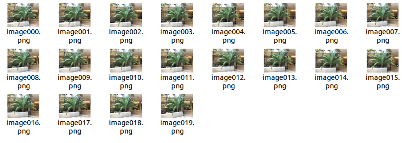
Input contains images with same resolution and their corresponding pose matrix. In addition, there's also the near bound the far bound of the scene.
The images can be seen as a Tensor with shape [H W 3], whose values fall between 0 to 255. But it will be divided by 255 to make them fall between 0 and 1.
Sometimes pose matrix is ambiguous(intrinsic or extrinsic). Here, pose matrix denotes extrinsic matrix(world to camera matrix).
Each image has a pose matrix like:
The column [x y z] in this matrix respectively denotes [right up back] in orthogonal camera coordinates.
The column [t] means the translation vector.
In
Data preprocess details
We focus mostly on the pose matrix.
1.Column modification
The rotate matrix given in LLFF dataset is in the form of [down right back] in default. It should be fixed to [right up back].(Coordinate doesn't change, just change its representation method, so translation vector doesn't need to modify in this step)
2.Scale by the bound
Review the NDC coordinates:
All axes in NDC is bounded between [-1, 1]. When the camera coordinate is transformed into NDC, we want to assume the near plane is at n=-1. So we should rescale the bounds and the translation vector.
What we do is as following:
bd_factor = 0.75sc = 1. if bd_factor is None else 1./(bds.min() * bd_factor)poses[:,:3,3] *= sc # scale the translation vectorbds *= scThe bound is set to about at n=-1.333 in case the bound wasn't conservative enough. When we hardcode the near to be n=-1, the scene will still be clipped in to NDC even if the actual bound is bigger than n=-1.333.
3.Recenter the pose
We want to normalize the orientation of the scene(that is the identity extrinsic matrix is looking at the scene). So what we need to do is applying the inverse of this average pose(c2w) transformation to the dataset.
In original dataset, exists:
If we applying a transformation to
What we need to do in code is applying the inverse of this average pose(c2w) transformation to all pose transformation:
poses = np.linalg.inv(avg_c2w) @ posesThe final situation is the world coordinate is fixed to be the average camera coordinate.
Render pipeline
1.Ray generation
In this part, the ray position is still in the camera coordinate(not NDC).
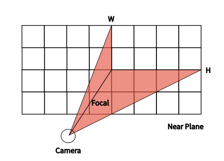
Now that we assume near plane is at n=-1, so the maximum translation on x axis is
Each ray corresponds to a certain pixel in the image.
x = [[-252., -251., -250., ..., 249., 250., 251.],[-252., -251., -250., ..., 249., 250., 251.],[-252., -251., -250., ..., 249., 250., 251.],...,[-252., -251., -250., ..., 249., 250., 251.],[-252., -251., -250., ..., 249., 250., 251.],[-252., -251., -250., ..., 249., 250., 251.]] / Focaly = [[ 189., 189., 189., ..., 189., 189., 189.],[ 188., 188., 188., ..., 188., 188., 188.],[ 187., 187., 187., ..., 187., 187., 187.],...,[-186., -186., -186., ..., -186., -186., -186.],[-187., -187., -187., ..., -187., -187., -187.],[-188., -188., -188., ..., -188., -188., -188.]] / Focalz = -np.ones_like(x)The vector mentioned above is still in camera coordinate. The train should use the rays in world coordinate. So we should transform the ray vector from camera coordinate to world coordinate.
Consider that the camera is at (0,0,0) in camera coordinate, so it just need to do the translation to get transformed into world coordinate.
Finally we get a tensor like [batch, ro+rd, H, W, 3]. Every image has H*W rays' origin and direction vector.
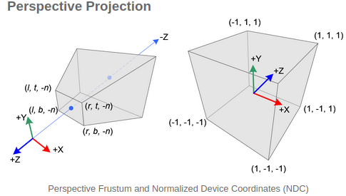
2.Normalized device coordinates
Now that
t = (rays_o[...,2] - (-1)) / rays_d[...,2]rays_o = rays_o + t[...,None] * rays_dThis new
Note that the eye coordinates are defined in the right-handed coordinate system, but NDC uses the left-handed coordinate system. That is, the camera at the origin is looking along -Z axis in eye space, but it is looking along +Z axis in NDC.(OpenGL Projection Matrix)
The rays in viewing frustum being transformed into NDC. In NDC, the near plane is at n=-1 and the far plane is at n=1.
Note that, as desired, t′ = 0 when t = 0. Additionally, we see that
The whole transform process and its proof can be seen in this link.
3. Network processing
Now we can make a conclusion that: when t'=0, ray is at near plane, when t'=1, ray is at far plane.
We can take samples by setting t' to get the points' position of the rays in NDC.
NeRF simultaneously optimizes two models, one coarser, one finer.
After we feed the sampled points' position and its direction to two networks, we will get two chunks of RGB values.
4. Volume Rendering Introduction
In original paper of NeRF, the modeling and proof of volume rendering is not fully included. This paper gives an partly reasonable introduction.
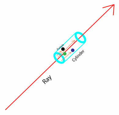
We assume light's length is
In the blue cylinder, the light collides with the particles. We make a hypothesis that all particles are the ball with the same size. We assume its radius is
If we look from the bottom of the blue cylinder, the area covered by one particle is
We also assume that the bottom area of the blue cylinder is
The number of particles in the cylinder is:
When
The covered proportion of the cylinder bottom is:
Light only gets through the uncovered area of the cylinder bottom, the intensity becomes:
The intensity difference is:
It can be transformed into a differential equation:
We define:
We can know that
The original equation becomes:
After we do an integration, we get:
When x=0, we know
We get:
We define:
We define a random variable
The final return color of the ray is the expectation of the color of the particle which blocks the light. We assume that the particle color at
Let
The original
which is the first equation in NeRF, where
5. Numerical calculation
In computer, we should construct a numerical integration.
Assume that the sampled points are
In the above proof, we make an assumption that
So the calculation for
which is the third equation in NeRF.
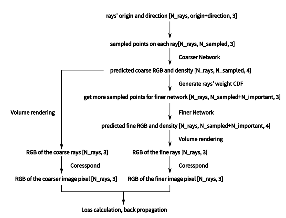
6. Overall pipeline
We generate the ray in camera coordinate, and transform it to world coordinate. Each ray correspond to a certain pixel in the image. Rays' origin and direction is the batch, certain pixel RGB value is the target.
Then comes the rendering.
We transform the rays' origin and direction in perspective frustum to NDC. And sample several points from each ray. ([N_ray, N_sample, 3])
Then we feed the xyz in NDC and viewing direction in NDC to the network, and finally we get its predicted density
We use volume rendering. Given predicted density
Optimization
We use N_samples number of points to train coarser network, use N_samples+N_important number of points to train fine network.
Two networks will output two images, whose losses are added together to optimize these two networks.
The result takes solely from the finer network, but coarser network also need to be trained.
The item
After volume rendering of the coarser image finishes, another bunch of important points will be sampled based on the weight CDF predicted by the coarser network. This is where the N_important number of sampled points come from.
In other words, coarser network is trained to help the stratified/hierarchical sampling for the finer network.
Misc
1.Pixel depth and disparity
In volume rendering process, considering the samples from one single ray, the point must have a high density if its weight takes a big value. So we think the weight of sampled point contribute to the evaluation of a pixel depth.
depth_map = torch.sum(weights * z_vals, -1)Every sampled point on one single ray has a weighted contribution to the pixel depth.
Disparity just takes its scaled reciprocal.
disp_map = 1./torch.max(1e-10 * torch.ones_like(depth_map), depth_map / torch.sum(weights, -1))2.White background
Render a scene with a white background just need a little modification in rgb_map.
# the ray with low accumulative weights means that# there is no high opacity.# so rgb value of that ray will be bigger than or equal to 1, means whitergb_map = rgb_map + (1.-acc_map[...,None])3.Render pose generation
The position of the camera is the key point for pose generation, because vector
c = np.dot(c2w[:3,:4], np.array([np.cos(theta), -np.sin(theta), -np.sin(theta*zrate), 1.]) * rads)The code use the parametric equation
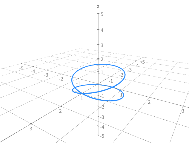
The path can be seen in this url.